Big O with a contact-list search you can count

If you know JavaScript arrays and loops, a contact search is a useful place to learn Big O because you can count the work before you need a stopwatch. Suppose an array contains 1,000 contacts, and the search compares a requested ID with each contact’s ID until it finds a match. Finding the first contact takes one comparison. Finding the last takes 1,000. A missing ID also takes 1,000.

The same function produced all three results. Its cost depends on the input, including the position of the requested contact. Big O describes how a chosen cost grows as the input gets larger. The MIT lecture transcript on algorithms and computation makes this distinction between an input size and the work an algorithm performs. For this search, the worst-case comparison count grows linearly with the number of contacts.

Make the work visible

Here is a small version you can run in a browser console or Node.js. The comparisons field is instrumentation for the example; a normal search function would usually return only the contact or its index.

function findContact(contacts, wantedId) {
  let comparisons = 0;
  for (const contact of contacts) {
    comparisons += 1;
    if (contact.id === wantedId) {
      return { contact, comparisons };
    }
  }
  return { contact: null, comparisons };
}

const contacts = Array.from({ length: 1000 }, (_, id) => ({ id }));
console.log(findContact(contacts, 0).comparisons);    // 1
console.log(findContact(contacts, 999).comparisons);  // 1000
console.log(findContact(contacts, -1).comparisons);   // 1000

The size variable, usually written as n, is the number of contacts. Each equality check is treated as a constant-cost operation because these IDs are bounded-size numbers. If the search compared arbitrarily long strings instead, the length and comparison rules for those strings could become another part of the cost model.

For the missing-ID case, doubling the array from 1,000 to 2,000 doubles the equality checks. That is a more useful observation than saying the first run took a particular number of milliseconds. Browser scheduling, CPU state, and other processes can change a timing result without changing the algorithm.

Best, worst, and average are different questions

The best successful lookup makes one comparison, while the worst successful or unsuccessful lookup makes n. An average needs a model of which queries occur. If every stored ID is equally likely and every query succeeds, the possible comparison counts are one through n, giving an average of (n + 1) / 2. For 1,000 contacts that is 500.5 comparisons, even though an individual query never performs half a comparison.

If a fraction p of queries misses, and successful queries remain uniform over positions, the expected count becomes (1 - p) * (n + 1) / 2 + p * n. At p = 0.2 and n = 1000, that is 600.4. A directory whose most frequently requested contacts are near the beginning can have a different average. The worst-case bound stays the same.

This distinction also separates an observed average from an expected value in a model. The formula is derived from stated probabilities; a measured average comes from an actual query sample. Neither automatically describes another application’s users. An empty list takes zero comparisons and returns no contact, which the implementation already handles without indexing a first element.

What O(n) actually promises

An upper bound of O(n) says the cost eventually stays below a constant multiple of n. More formally, there are positive constants c and n₀ such that the cost is at most c × n whenever n ≥ n₀.

This definition ignores fixed startup costs and constant factors when describing long-term growth. A search doing 3n + 12 simple operations is O(n), as is one doing n such operations. The first can still be noticeably slower. Complexity analysis does not erase constant factors from an actual product.

For the worst-case linear search above, Θ(n) is the tighter statement: the number of comparisons is bounded both above and below by constant multiples of n. Saying O(n²) would also be a valid upper bound, but it would hide the fact that this function grows more slowly than a quadratic search. In everyday discussions, people often use Big O when they mean the tight growth rate. It helps to know which claim the notation actually makes.

View full-size image ↗

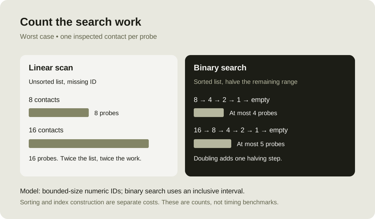
The diagram compares worst-case equality or three-way ordering probes under a simplified model. A real binary-search implementation may perform more than one primitive comparison per probe. That distinction changes a constant factor, while the halving pattern remains.

Why sorted contacts change the search

If the contacts are sorted by numeric ID, binary search can inspect the middle and discard half of the remaining range. After one probe, roughly n/2 candidates remain. After two, roughly n/4 remain. After k, the remaining range is roughly n/2ᵏ.

The range reaches a constant size when 2ᵏ is about n, giving k about log₂ n. A standard binary search therefore has O(log n) worst-case search time. For an array of 1,000 items, a conventional inclusive-range implementation needs at most 10 middle-element probes. Increasing the array to 2,000 raises that bound to 11.

There is a condition attached to this improvement: the data must already be sorted by the same key and ordering used by the search. Sorting an arbitrary array for one lookup can cost more than scanning it once. If you will make many lookups and the list changes infrequently, sorting once and searching repeatedly becomes a different tradeoff.

Also consider the query itself. An array sorted by ID does not help a request such as “show contacts whose notes contain architect.” That predicate is unrelated to the ordering. Choosing an algorithm starts with defining the operation you need to support.

You can make the binary-search probes visible too. This version uses an inclusive interval and returns any matching ID; the example assumes IDs are unique.

function findSortedContact(contacts, wantedId) {
  let left = 0, right = contacts.length - 1, probes = 0;
  while (left <= right) {
    const middle = left + Math.floor((right - left) / 2);
    const contact = contacts[middle];
    probes += 1;
    if (contact.id === wantedId) return { contact, probes };
    if (contact.id < wantedId) left = middle + 1;
    else right = middle - 1;
  }
  return { contact: null, probes };
}

console.assert(findSortedContact(contacts, 999).probes === 10);
console.assert(findSortedContact(contacts, 1000).probes === 10);
console.assert(findSortedContact([], 1).probes === 0);

The sorted ordering lets each failed probe discard the midpoint and one side of it. On an unsorted array, that discard has no justification, so the same code can miss an existing ID. Checking sortedness before every lookup would itself cost O(n); validate or maintain that property at the point where the collection changes.

An index moves some work earlier

A hash table offers another option for exact-ID lookups. You can first construct a mapping from ID to contact, then query that mapping. Under the usual hashing assumptions, lookups take expected O(1) time, and building the table takes expected O(n) time, as developed in Open Data Structures on hash tables. The table also consumes additional memory. The model assumes that the hash function spreads keys sufficiently evenly and that the number of entries per bucket stays bounded on average. Colliding keys still need to be distinguished. If many keys accumulate in one bucket, a lookup can inspect a long chain; expected O(1) is not a promise about every individual query.

JavaScript’s Map is convenient for this pattern:

const byId = new Map(contacts.map(contact => [contact.id, contact]));
const result = byId.get(999);

Do not turn that example into a language-level promise that every Map.get operation is worst-case O(1). The JavaScript specification requires average access time to be sublinear in the number of elements; implementations can satisfy that requirement using different data structures. The expected constant-time statement belongs to a hash-table model with stated assumptions.

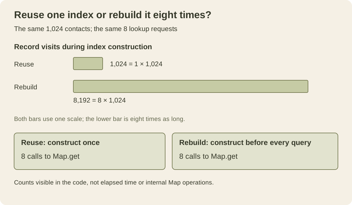
There are ordinary application details too. Duplicate IDs cause later entries to replace earlier entries in this construction. Adding or removing a contact requires updating the index. Rebuilding the entire index during every render revisits all n contacts to save a single O(n) scan. An index helps when its lifecycle matches the workload.

Count the index lifetime, not only one lookup

Suppose a fixed snapshot contains 1,024 contacts and serves eight lookups. Building an index once visits 1,024 source records; rebuilding it for every lookup visits 8,192 records. Both designs issue eight get calls. These are counts of actions visible in the program, not measurements of the hidden work inside Map or elapsed time.

View full-size image ↗

function buildContactIndex(snapshot) {
  const index = new Map();
  let recordsVisited = 0;
  for (const contact of snapshot) {
    recordsVisited += 1;
    index.set(contact.id, contact);
  }
  return { index, recordsVisited };
}

const snapshot = Array.from({ length: 1024 }, (_, id) => ({ id }));
const queryIds = [0, 1, 7, 31, 255, 511, 999, 1023];
const shared = buildContactIndex(snapshot);
for (const id of queryIds) shared.index.get(id);
let rebuiltVisits = 0;
for (const id of queryIds) {
  const rebuilt = buildContactIndex(snapshot);
  rebuiltVisits += rebuilt.recordsVisited;
  rebuilt.index.get(id);
}
console.assert(shared.recordsVisited === 1024);
console.assert(rebuiltVisits === 8192);

Under an expected constant-time hash-table model, one build followed by q lookups costs expected O(n + q), while rebuilding for each lookup costs expected O(qn + q). The actual JavaScript implementation still has the specification’s broader access-time contract. Keep the abstract data-structure analysis distinct from what the language guarantees.

Reusing an index creates a maintenance obligation. If a contact’s ID changes, mutating the object does not move its entry to a new map key. A deleted contact can remain reachable through a stale index. Update the list and index together, or rebuild when a new snapshot is accepted. Which policy is simpler depends on how often the data changes relative to how often it is searched.

The index consumes memory for its entries. It may point to the existing contact objects rather than copy them, but sharing those references also means later object mutations are visible through the map. Performance and state ownership need to be designed together; the lookup’s isolated complexity does not settle either question.

A small experiment to try

Run the instrumented linear search with arrays of 8, 16, 32, and 64 contacts. For each size, request the first ID, the last ID, and an absent ID. Write down the counts before running the code. Then replace the search with binary search on the sorted numeric IDs and count middle-element probes.

Keep the same definition of an operation when comparing runs. If you count loop iterations in one implementation and every primitive comparison in the other, label those columns separately. Both measurements can be useful, but they answer different questions.

Once the counts match your prediction, measure elapsed time over repeated runs. On small arrays, a linear scan may be competitive because it is simple and reads adjacent memory. That result does not disprove the asymptotic analysis. It tells you the tested input sizes, implementation, and machine have not made growth rate the only relevant factor.

For a contact picker with a few dozen entries, the simplest scan may be enough. For a large directory queried repeatedly, the indexing strategy deserves attention. Write down the input size, the query pattern, and the update frequency before choosing between them.